Scattering due to edge imperfections in topological insulators in the uniform magnetic field

Full Text

1. Introduction

Topological insulators (TIs) are novel materials that cannot be continuously converted into semiconductors or conventional insulators. They are distinguished by gapless edge or surface states and a complete insulating gap in the bulk. Time reversal (TR) symmetry protects the edge (in 2D TIs) or surface (in 3D TIs) states from elastic scattering. Error-tolerant quantum computing[1, 2] and low-power circuits [3] are two potential uses for TI.

The features of TIs have piqued the interest of the scientific community due to experimental observations of surface states[4] in Bi₂Se₃ crystals and transport by edge states in HgTe quantum wells (QW)[5]. The edge states are either 2D states on the boundaries of 3D TI (as in the case of Bi₂Se₃ [6]) or 1D states on the boundaries of 2D TI (e.g., HgTe quamtum well). With the exception of HgTe [7], 2D and 3D TI samples are typically comprised of distinct compounds. Other realizations of 1D topologically protected states are found on step edges[8, 9] and on the edges between 3D TI surfaces[10].

The most striking feature of edge states in 2D TI is that, as a result of spin-momentum locking, the scattering event$—$which, in the case of a 2D TI edge, is always a back-scattering inevitably involves the quasiparticle’s spin flipping. Consequently, the elastic scattering of the edge states is prohibited in the absence of magnetic impurities or other TR - violating contributions. This is the well-known manifestation of TR - symmetry in these kinds of systems [11]. Another important peculiarity of TI compounds is the pronounced spin-orbit interaction (SOI), [12, 13].

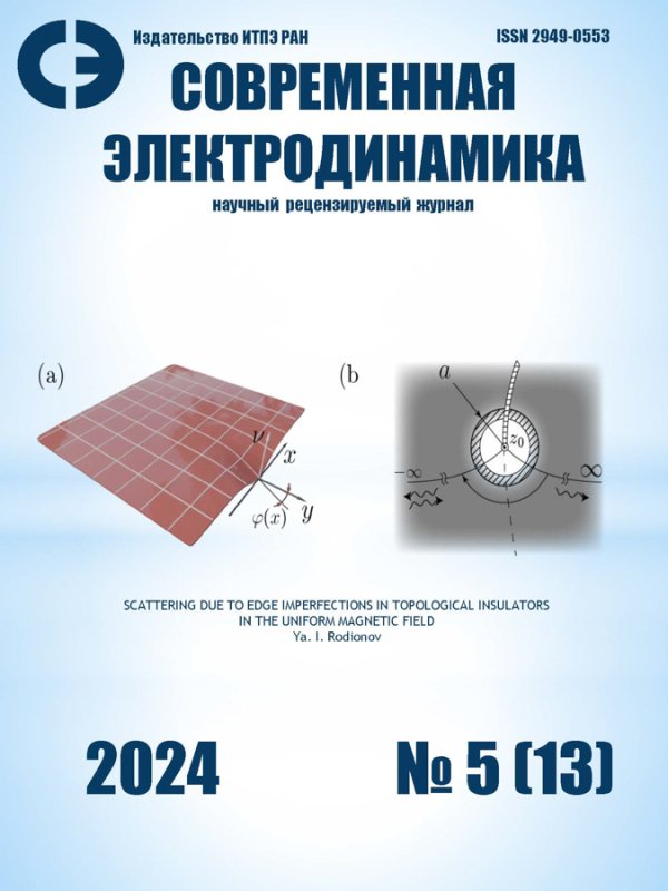
In paper [14], we introduced a model edge Hamiltonian describing the influence of SOI on edge imperfections. The edge imperfection is controlled by the deformation angle profile (see Fig. 1(a)). The elastic scattering becomes possible in the presence of the uniform magnetic field orthogonal to the edge. This model predicts an interesting effect. At not very strong magnetic fields the reflection coefficient exhibits pronounced oscillations as a function of magnetic field. In this paper we expand our study and discover new type of quantum oscillations of the reflection coefficient for another general type of potentials at Zeeman energies close to the energy of quasiparticles. We also extend the previous study on the deformation potential of yet another analytical structure. As usual, for the smooth deformation profiles the poweful Pokrovsky-Khalatnikov method [15] is used to obtain the analytic reflection amplitude with pre-exponential accuracy.

Рис. 1: A schematic illustration of a geometric imperfection on the edge of a 2D topological insulator sample

The paper is organized as follows. Section 1 is dedicated to the initial model and main approximations of the problem. Section 2 introduces the principle points of semiclassical Pokrovsky-Khalatnikov procedure. Section 3 deals with its application to the an important class of scattering potentials for slow moving edge excitations. Section 4 generalizes the previous treatment of the same problem to the wider class of potentials. Section 5 discusses the exact solution of the magnetic-field-free problem and presents the perturbation (in magnetic field) theory, as well as the matching of perturbative and semiclassical limit. We summarize the results in Section 6.

1 The model

The Hamiltonian of a 2D TI for the edge excitations has the following form [16]:

$\widehat{H}=H_0+H_{so}\mathrm{,}{H}_0=v_{F0}{\widehat{p}}_x{\widehat{\sigma }}_y\mathrm{,}{H}_{so}=\alpha \overrightarrow{\sigma }\times \overrightarrow{p}\cdot \overrightarrow{\nu }\mathrm{.}$ (1)

Here, 𝐻₀ is the effective Hamiltonian of edge states moving along x-axis (y=0) and $\overrightarrow{\sigma }\mathrm{<mo>=</mo><mo\; stretchy="false">(</mo>}{\sigma }_x\mathrm{,}{\sigma }_y\mathrm{,}{\sigma }_z\mathrm{<mo\; stretchy="false">)</mo>}$ are Pauli matrices in the spin 1/2 basis and 𝑣_𝐹0 is a bare Fermi velocity.

The spin-orbital interaction Hamiltonian 𝐻_𝑠𝑜 is derived in paper [17] where a 2D electron gas was addressed; $\overrightarrow{p}$ is electron’s momentum, 𝜈 is a unit normal to the surface of the TI (or to an interface in a heterostructure), and 𝛼 is Rashba parameter. The latter depends on the external electric field (the gate voltage)[12, 13] as well as the material. The former causes the splitting in energy bands due to electron’s spin (Rashba splitting), which is pronounced in energy band structure of TI materials [13, 18].

It is crucial to note here how the normal vector’s 𝜈 direction should be fixed. Essentially, the right direction may be inferred from the original TI Hamiltonian, which we won’t show here. Nevertheless, we rely on article [18], which demonstrates that a TI’s Fermi velocity increases as Rashba’s coefficient 𝛼 decreases. The orientation shown in Fig. 1(a) corresponds to the correct direction of 𝜈, as we will see below.

Let us consider a deformation at the edge, as depicted in Fig. 1(a). The tangent profile of the sample edge is bent in 𝑦𝑧 plane and determined by the function 𝜑(𝑥). This deformation leads to a transformed spin-orbit interaction

$H_{so}=-\alpha {\widehat{p}}_x{\widehat{\sigma }}_y+\widehat{U}x,\widehat{U}x=\frac{\alpha }{2}\left[{\widehat{p}}_x\varphi \right(x)+\varphi (x\left){\widehat{p}}_x\right]{\sigma }_z$ (2)

for smooth and shallow defects ( $\varphi \mathrm{<mo\; stretchy="false">(</mo>}x\mathrm{<mo\; stretchy="false">)</mo>}\ll 1$ ). To preserve the hermicity of the initial SOI Hamiltonian (1) we introduced the anti commutator (due to the 𝑥 -coordinate dependence of the normal vector 𝜈). The first term in (2), $-\alpha {\widehat{p}}_x{\widehat{\sigma }}_y$ is a simple renormalization of the Fermi velocity, as we see from the initial Hamiltonian (1). The latter term in (2) is supposed to be treated as an elastic potential profile of the problem. In what follows, it would be convenient to incorporate the parameter 𝛼 in the profile deformation function: $\phi \mathrm{<mo>=</mo>}\alpha \varphi$.

The potential profile function $\widehat{U}$ in (2) alone will not cause backscattering of the edge states, since $\widehat{U}$ does not break TR - symmetry. However, that is not the case in the presence of the uniform magnetic field, since the latter does break the TR - symmetry. Therefore, we apply magnetic field in the vertical direction (𝑧 -axis) (i.e. orthogonal to the plane of the TI sample). The suitable gauge of vector-potential is as follows: $\overrightarrow{A}\mathrm{<mo>=</mo><mo\; stretchy="false">(</mo>}\mathcal{H}y\mathrm{,0,0<mo\; stretchy="false">)</mo>}$. We note here, that 𝑦 - coordinate remains constant in our case $y\mathrm{<mo>=</mo>}\text{c}onst$ /. Therefore, it can be safely put equal to zero (alternatively, for constant 𝑦 the vector potential can be removed from Dirac’s equation via elementary gauge transformation). Thus, the only change of the Hamiltonian brought by the magnetic field is the addition of a Zeeman term:

${\widehat{H}}^{1D}\mathrm{<mo\; stretchy="false">(</mo>}x\mathrm{<mo\; stretchy="false">)</mo><mo>=</mo>}{v}_F{\widehat{p}}_x{\sigma }_y+\mu {\sigma }_z+\widehat{U}\mathrm{<mo\; stretchy="false">(</mo>}x\mathrm{<mo\; stretchy="false">)</mo>.}$ (3)

Here, $v_F\mathrm{<mo>=</mo>}{v}_{F0}-\alpha$ is a renormalized Fermi velocity and $\mu \mathrm{<mo>=</mo>}{\mu }_{B}g\mathcal{H}$, 𝑔 is the edge electron’s g-factor [19]. We consider the application of the transverse magnetic field only. As shown in [20], the in-plane magnetic field can be eliminated by a gauge transformation of the electron field operators.

As a result, we end up solving the scattering problem for the following equation:

$\left[v_F{\widehat{p}}_x{\sigma }_y+\mu {\sigma }_z+\widehat{U}\mathrm{<mo\; stretchy="false">(</mo>}x\mathrm{<mo\; stretchy="false">)</mo>}\right]\psi \mathrm{<mo\; stretchy="false">(</mo>}x\mathrm{<mo\; stretchy="false">)</mo><mo>=</mo>}\epsilon \psi \mathrm{<mo\; stretchy="false">(</mo>}x\mathrm{<mo\; stretchy="false">)</mo>}$ (4)

As one readily sees, even in the absence of deformation potential $\widehat{U}\mathrm{<mo\; stretchy="false">(</mo>}x\mathrm{<mo\; stretchy="false">)</mo>}$ the Zeeman term $\mu {\sigma }_z$ leads to a gap in the spectrum of edge state of the width $\mu$. Therefore, the unbound states always obey the condition:

$\epsilon \mathrm{<mo>></mo>}\mu \mathrm{.}$ (5)

2 Methods

The Dirac equation (4) comprises two first order differential equations on the pair 𝜓 = (𝜓₁, 𝜓₂). The most convenient approach to its analysis surprisingly happens to be the reduction of system (4) to a 2nd order differential equation on a single function 𝜓₁:

$2{\hslash }^2\text{}\left({\phi }^2\text{}+\text{}1\right)\text{}\alpha {\psi }_{{1^{\prime }}^{\prime }}\text{}\text{}+\text{}2i\hslash \text{}\left[{\hslash }^2\text{}\left({\phi }^2\text{}+\text{}1\right){{\phi }^{\prime }}^{\prime }\text{}+\text{}\phi \alpha \left(2\mu \text{}-\text{}3i\hslash {\phi }^{\prime }\right)\right]\text{}{\psi }_{1^{\prime }}+\left[\frac{1}{2}\alpha \beta \mathrm{<mo\; stretchy="false">(</mo>}\alpha -2i\hslash {\phi }^{\text{'}}\mathrm{<mo\; stretchy="false">)</mo>}+4\epsilon {\hslash }^2\phi {{\phi }^{\prime }}^{\prime }\right]{\psi }_1\mathrm{<mo>=</mo>0,}$ (6)

${\psi }_2\mathrm{<mo>=</mo>}\frac{2\hslash \left({\phi }^2+1\right){\psi }_{1^{\prime }}-i{\psi }_1\phi \beta \mathrm{<mo\; stretchy="false">(</mo>}x\mathrm{<mo\; stretchy="false">)</mo>}}{\alpha \mathrm{<mo\; stretchy="false">(</mo>}x\mathrm{<mo\; stretchy="false">)</mo>}}\mathrm{.}$ (7)

Here $\alpha \mathrm{<mo\; stretchy="false">(</mo>}x\mathrm{<mo\; stretchy="false">)</mo><mo>=</mo>2<mo\; stretchy="false">(</mo>}\mu +\epsilon \mathrm{<mo\; stretchy="false">)</mo>}-i\hslash {\phi }^{\prime }\mathrm{,}\beta \mathrm{<mo\; stretchy="false">(</mo>}x\mathrm{<mo\; stretchy="false">)</mo><mo>=</mo>2<mo\; stretchy="false">(</mo>}\mu -\epsilon \mathrm{<mo\; stretchy="false">)</mo>}+i\hslash {\phi }^{\prime }$.

The derivation of (6) is straightforward and presented in [14]. Due to its complexity, differential equation (6) cannot be solved exactly. We are going to approach it from two different limits:

(i) semiclassical approximation, corresponding to the smooth deformation 𝜙(𝑥) of the edge;

(ii) perturbation theory in magnetic field strength (Zeeman energy) 𝜇. For the wide class of potentials we are going to show how these two approaches match.

2.1 Semiclassical approximation

First, we need to determine the small parameter of the problem. Physically speaking, semiclassical treatment corresponds to the case of smooth (on the scale of de Broglie wavelength) deformation potential $\phi$ (𝑥). The characteristic scale at which the potential changes is denoted as 𝑎₀. The smoothness of the potential then means:

$\frac{\lambda }{a_0}\equiv \frac{\hslash v_F}{\epsilon a_0}\ll 1\mathrm{<mo\; stretchy="false">(</mo>}semiclassicalapproximation\mathrm{<mo\; stretchy="false">)</mo>}$ (8)

The semiclassical scattering in the problem is structured in a way that, as we will see in the study that follows, the semiclassical momentum never vanishes on the real axis in view of condition (5), rendering the scattering an over-barrier event. Therefore, Pokrovsky-Khalatnikov [15] (P-Kh) method seems to be the most adequate approach to the task. For convenience, we use $\hslash \mathrm{<mo>=</mo>}{v}_F\mathrm{<mo>=</mo>1}$ units system throughout the rest of the paper, restoring them when needed.

2.2 Pokrovsky-Khalatnikov approach

The concept of the method can be condensed to the following key steps (see also the work by M. Berry [21]):

(i) Perform the analytical continuation of the semiclassical solution into the complex plane along a so called anti-Stokes line, $\text{I}m{\displaystyle {\int }_{z_0}^z}k\mathrm{<mo\; stretchy="false">(</mo>}z\mathrm{<mo\; stretchy="false">)</mo>}dz\mathrm{<mo>=</mo>0}$ where 𝑘(𝑧) is the semiclassical momentum and $z_0$ is the so called turning point in the complex plane.

(ii) Construct the exact solution of the Schrödinger equation around the turning point 𝑧₀, when the differential equation substantially simplifies due to the Taylor-expansion of momentum 𝑘(𝑧).

(iii) Determine the exact solution’s asymptotics on the anti-Stokes lines that extend from the turning point to the left and right.

(iv) Presuming that there is a non-empty intersection of the range of existance of the asymptotics of exact and semiclassical solutions (the striped region in Fig. 1(b)) match the semiclassical and exact solutions in the mentioned range on anti-Stokes lines.

(v) Build an analytic continuation from the anti-Stokes line running to −∞ on the real axis 𝜓(𝑧) → 𝜓(𝑥).

We are going to implement the outlined program step by step explaining all the nuances in the rest of the paper.

2.3 Semiclassical solution

Let us make the exponential substitute $\psi \to e^{iS\mathrm{<mo>/</mo>}\hslash }$ for the wave function and employ the standard semiclassical expansion in the powers of ℏ adapted to the equation (6):

$\psi \mathrm{<mo>=</mo>}\left(\begin{array}{c}{\psi }_1\\ {\psi }_2\end{array}\right)\mathrm{,}{\psi }_{\mathrm{1,2}}\mathrm{<mo>=</mo>}\exp \left(\frac{i{S}_0}{\hslash }+i{S}_{\mathrm{1,2}}+\mathrm{...}\right)\mathrm{.}$ (9)

In the zeroth order in ℏ (i.e. discarding all terms with derivatives of $\phi$ in Eq. 6) we obtain the following expression for 𝑆₀ [14]:

$S_0\mathrm{<mo\; stretchy="false">(</mo>}x\mathrm{<mo\; stretchy="false">)</mo><mo>=</mo>}{\displaystyle \int }{q}_{\pm }\mathrm{<mo\; stretchy="false">(</mo>}{x}^{\prime }\mathrm{<mo\; stretchy="false">)</mo>}d{x}^{\prime }\mathrm{,}$ (10)

$q_{\pm }\mathrm{<mo>=</mo>}\frac{-\mu \phi \pm p}{{\phi }^2+1}\mathrm{,}p\mathrm{<mo>=</mo>}\sqrt{{\epsilon }^2\mathrm{<mo\; stretchy="false">(</mo>}{\phi }^2+\mathrm{1<mo\; stretchy="false">)</mo>}-{\mu }^2}\mathrm{,}$ (11)

where $q_{\pm }$ is interpreted as semiclassical momentum. The regular branch of 𝑝 is chosen in such a way that $p\underset{x\to +\infty }{\to }\sqrt{{\epsilon }^2-{\mu }^2}$. Then, retaining the next terms of order ℏ (𝑆_1,2 in the substitute (9)), and plugging it back in (6) we obtain the pre-exponential semiclassical terms for the wave function 𝜓:

$\begin{array}{l}{\psi }_{\mathrm{1,}\pm }\left(x\right)={\xi }_{\mathrm{1,}\pm }\left(x\right)e^{\frac{i}{\hslash }\int q_{\pm }dx}{\xi }_{\mathrm{1,}\pm }=\sqrt{\pm q_{\pm }[1\pm \frac{\phi \epsilon }{p}]}\\ {\psi }_{\mathrm{2,}\pm }\left(x\right)=-i{\psi }_{\mathrm{1,}\pm }\frac{\epsilon \phi \mp p}{\epsilon +\mu }\mathrm{.}\end{array}$ (12)

The square roots entering the definition of ${\xi }_{\mathrm{1,}\pm }$ are assumed to be positive at 𝑥 → +∞. To clear out which of the solutions corresponds to the right (left) moving carriers we need semiclassical currents:

$j_{\pm }\equiv {\psi }_{\pm }^{†}{\sigma }_y{\psi }_{\pm }=\frac{2q_{\pm }}{p}(\epsilon -\mu ),j_{\pm }\underset{x\to \infty }{=}\pm 2(\epsilon -\mu ).$ (13)

In the last equation in (13) we take into account that deformation function $\phi$ (𝑥) → 0 at 𝑥 → ±∞

2.4 Transformation from Dirac to Schrödinger equation.

To make the analogy between Dirac equation Eq. 6 and Schrödinger equation explicit, we get rid of the first derivative in (6) via a standard substitute [22]. Therefore, the equation is transformed according to:

${{\psi }^{\prime }}^{\prime }\mathrm{<mo\; stretchy="false">(</mo>}x\mathrm{<mo\; stretchy="false">)</mo>}+\eta \mathrm{<mo\; stretchy="false">(</mo>}x\mathrm{<mo\; stretchy="false">)</mo>}{\psi }^{\prime }\mathrm{<mo\; stretchy="false">(</mo>}x\mathrm{<mo\; stretchy="false">)</mo>}+\kappa \mathrm{<mo\; stretchy="false">(</mo>}x\mathrm{<mo\; stretchy="false">)</mo>}\psi \mathrm{<mo\; stretchy="false">(</mo>}x\mathrm{<mo\; stretchy="false">)</mo><mo>=</mo>0}\Rightarrow$

${\theta }^{\text{'}\text{'}}(x)+{\pi }^2(x\left)\theta \right(x)=0\text{\hspace{0.33em}(Schrödinger equation)}$ (14)

$\theta \mathrm{<mo\; stretchy="false">(</mo>}x\mathrm{<mo\; stretchy="false">)</mo><mo>=</mo>}{e}^{\frac{1}{2}{\displaystyle \int }\eta \mathrm{<mo\; stretchy="false">(</mo>}t\mathrm{<mo\; stretchy="false">)</mo>}dt}\psi \mathrm{<mo\; stretchy="false">(</mo>}x\mathrm{<mo\; stretchy="false">)</mo>,}$ (15)

${\pi }^2\mathrm{<mo\; stretchy="false">(</mo>}x\mathrm{<mo\; stretchy="false">)</mo><mo>=</mo>}\kappa \mathrm{<mo\; stretchy="false">(</mo>}x\mathrm{<mo\; stretchy="false">)</mo>}-\frac{1}{2}{\eta }^{\prime }\mathrm{<mo\; stretchy="false">(</mo>}x\mathrm{<mo\; stretchy="false">)</mo>}-\frac{1}{4}{\eta }^2\mathrm{<mo\; stretchy="false">(</mo>}x\mathrm{<mo\; stretchy="false">)</mo>.}$ (16)

The expression for 𝜋²(𝑥) is quite cumbersome. Nevertheless, its is important, since it plays the role of the semiclassical momentum in the problem. Therefore, it is instructive to write down 𝜂(𝑥) and 𝜋²(𝑥) discarding all the derivatives of the potential field $\phi$ (𝑥) (zeroth semiclassical approximation) as well as semiclassical solution. This way the connection with the initial semiclassical relations (10), (11) becomes transparent:

$\eta \mathrm{<mo\; stretchy="false">(</mo>}x\mathrm{<mo\; stretchy="false">)</mo><mo>=</mo>}\frac{2i}{\hslash }\frac{\mu \phi \mathrm{<mo\; stretchy="false">(</mo>}x\mathrm{<mo\; stretchy="false">)</mo>}}{{\phi }^2\mathrm{<mo\; stretchy="false">(</mo>}x\mathrm{<mo\; stretchy="false">)</mo>}+1}\mathrm{,}{\pi }^2\mathrm{<mo\; stretchy="false">(</mo>}x\mathrm{<mo\; stretchy="false">)</mo><mo>=</mo>}\frac{{\epsilon }^2\mathrm{<mo\; stretchy="false">(</mo>}{\phi }^2+\mathrm{1<mo\; stretchy="false">)</mo>}-{\mu }^2}{{\mathrm{<mo\; stretchy="false">(</mo>}{\phi }^2+\mathrm{1<mo\; stretchy="false">)</mo>}}^2}$ (17)

${\theta }_{\pm }\mathrm{<mo\; stretchy="false">(</mo>}x\mathrm{<mo\; stretchy="false">)</mo><mo>=</mo>}\frac{1}{\sqrt{\pi \mathrm{<mo\; stretchy="false">(</mo>}x\mathrm{<mo\; stretchy="false">)</mo>}}}\exp \left(\pm i{\displaystyle {\int }_{x_0}^x}\pi \mathrm{<mo\; stretchy="false">(</mo>}t\mathrm{<mo\; stretchy="false">)</mo>}dt\right)\mathrm{.}$ (18)

In the last equation point 𝑥₀ needs to be chosen on the real axis. This way both functions ${\theta }_{\pm }$ have the same modulus. Apart from this 𝑥₀ is quite arbitrary and is picked from convenience considerations.

3 The reflection coefficient for the slow edge excitations

Now we would like to address quite a striking case of the over-barrier scattering in TI insulator. Suppose, the energy of the edge excitations is close to the Zeeman gap 𝜇, so that the condition

$\mathrm{<mo>|</mo>}\epsilon -\mu \mathrm{<mo>|</mo>}\ll \epsilon$ (19)

is satisfied. It corresponds to the case of carriers with small momenta $v_{F}p\ll \mu$. This ought to be a realistic situation at temperatures much lower than Zeeman energy $\mu$. As we are going to see, this situation also leads to a specific analytic structure of the momentum $\pi \mathrm{<mo\; stretchy="false">(</mo>}z\mathrm{<mo\; stretchy="false">)</mo>}$. Indeed, let us rewrite momentum $\pi \mathrm{<mo\; stretchy="false">(</mo>}z\mathrm{<mo\; stretchy="false">)</mo>}$, defined in Eq. 17 in a slightly different form:

$\pi \mathrm{<mo\; stretchy="false">(</mo>}z\mathrm{<mo\; stretchy="false">)</mo><mo>=</mo>}\frac{\epsilon \sqrt{{\phi }^2\mathrm{<mo\; stretchy="false">(</mo>}z\mathrm{<mo\; stretchy="false">)</mo>}+\frac{{\epsilon }^2-{\mu }^2}{{\epsilon }^2}}}{{\phi }^2\mathrm{<mo\; stretchy="false">(</mo>}z\mathrm{<mo\; stretchy="false">)</mo>}+1}\mathrm{.}$ (20)

The last formula, in view of condition (19), shows that function $\pi \mathrm{<mo\; stretchy="false">(</mo>}z\mathrm{<mo\; stretchy="false">)</mo>}$ has two coalescent branch points positioned near the complex root of $\phi \mathrm{<mo\; stretchy="false">(</mo>}{z}_0\mathrm{<mo\; stretchy="false">)</mo><mo>=</mo>0}$.

The semiclassical condition breaks down near these two coalescent branch points and we can employ step 2 from P-Kh method. We expand the semiclassical momentum near the point $z_0$, as follows:

${\pi }^2\mathrm{<mo\; stretchy="false">(</mo>}{z}_0+\zeta \mathrm{<mo\; stretchy="false">)</mo><mo>=</mo>}-{\epsilon }^2\frac{{\zeta }^2}{a^2}+2\delta \epsilon \epsilon \mathrm{,}$ (21)

where $\zeta \mathrm{<mo>=</mo>}z-z_0$. Here, parameter $a$ can be strictly speaking, complex. However, its modulus sets the characteristic scale of change of the potential. Therefore, one may assume that $\mathrm{<mo>|</mo>}a\mathrm{<mo>|</mo>}\sim a_0$, where $a_0$ is the scale of the deformation introduced in Eq. (8). This way, the Dirac equation (6) is turned into parabolic cylinder equation:

${\psi }_1^{\text{'}\text{'}}-{\epsilon }^2\left(\frac{{\zeta }^2}{a^2}-\frac{2\delta \epsilon }{\epsilon }\right){\psi }_1\mathrm{<mo\; stretchy="false">(</mo>}\zeta \mathrm{<mo\; stretchy="false">)</mo><mo>=</mo>0.}$ (22)

The anti-Stokes directions are given by the equation

$\text{I}m{\displaystyle {\int }_0^{\zeta }}\pi \mathrm{<mo\; stretchy="false">(</mo>}t\mathrm{<mo\; stretchy="false">)</mo>}dt\underset{\zeta \to \infty }{\mathrm{<mo>=</mo>}}\epsilon \text{R}e\frac{{\zeta }^2}{2a}\mathrm{<mo>=</mo>0}\Rightarrow \text{a}rg\zeta \mathrm{<mo>=</mo>}\frac{\pi }{4}+\frac{\text{a}rga}{2}+\pi n\mathrm{,}n\in \mathbb{Z}\mathrm{.}$ (23)

As a result, we choose the anti-Stokes lines with angles $-\pi \mathrm{<mo>/</mo>4}+\text{a}rga\mathrm{<mo>/</mo>2}$ and $-3\pi \mathrm{<mo>/</mo>4}+\text{a}rga\mathrm{<mo>/</mo>2}$. Substituting (21) into semiclassical expressions (10), (12) we obtain the semiclassical solution in the vicinity of point $z_0$ 

$\begin{array}{ll}{\psi }_{\mathrm{<mo><</mo>,}+}\mathrm{<mo\; stretchy="false">(</mo>}s\mathrm{<mo\; stretchy="false">)</mo>}\hfill & \mathrm{<mo>=</mo>}\sqrt{2}{\left[\text{}\frac{2s}{\gamma \text{}-\text{}1}\text{}\right]}^{\frac{\gamma }{2}-1}\text{}\text{}\text{}{e}^{-\frac{i{s}^2}{2}-\frac{i\pi \gamma }{8}-\frac{i\pi }{4}}{\mathrm{<mo\; stretchy="false">[</mo><mo\; stretchy="false">(</mo>}\gamma \text{}-\text{}\mathrm{1<mo\; stretchy="false">)</mo>}e\mathrm{<mo\; stretchy="false">]</mo>}}^{\frac{\gamma -1}{4}}\mathrm{,}{\psi }_{\mathrm{<mo><</mo>,}-}\mathrm{<mo\; stretchy="false">(</mo>}s\mathrm{<mo\; stretchy="false">)</mo><mo>=</mo>}\sqrt{2}{\left[\text{}\frac{2s}{\gamma \text{}-\text{}1}\text{}\right]}^{-\frac{\gamma }{2}}\text{}\text{}\text{}{e}^{\frac{i{s}^2}{2}+\frac{i\pi \gamma }{8}-\frac{i\pi }{2}}{\mathrm{<mo\; stretchy="false">[</mo><mo\; stretchy="false">(</mo>}\gamma \text{}-\text{}\mathrm{1<mo\; stretchy="false">)</mo>}e\mathrm{<mo\; stretchy="false">]</mo>}}^{-\frac{\gamma -1}{4}}\hfill \\ {\psi }_{\mathrm{<mo>></mo>,}+}\mathrm{<mo\; stretchy="false">(</mo>}s\mathrm{<mo\; stretchy="false">)</mo>}\hfill & \mathrm{<mo>=</mo>}\sqrt{2}{\left[\frac{2s}{\gamma \text{}-\text{}1}\right]}^{\frac{\gamma }{2}-1}{e}^{\frac{i{s}^2}{2}+\frac{i\pi \gamma }{8}-\frac{i\pi }{2}-\frac{\gamma -1}{4}}{\mathrm{<mo\; stretchy="false">[</mo><mo\; stretchy="false">(</mo>}\gamma \text{}-\text{}\mathrm{1<mo\; stretchy="false">)</mo>}e\mathrm{<mo\; stretchy="false">]</mo>}}^{\frac{\gamma -1}{4}}\hfill \end{array}$ (24)

Now, to proceed further we need to find exact solutions of Eq. (22)

3.1 Exact solution at the double branch point. Match with semiclassical wave functions.

Introducing variable change: $\zeta \mathrm{<mo>=</mo>}\sqrt{a\mathrm{<mo>/</mo>}\epsilon }s{e}^{-i\pi \mathrm{<mo>/</mo>4}}$, we obtain the differential equation

${\psi }_1^{\text{'}\text{'}}+\mathrm{<mo\; stretchy="false">(</mo>}{s}^2-2i\delta \epsilon a\mathrm{<mo>/</mo>}\epsilon \mathrm{<mo\; stretchy="false">)</mo>}{\psi }_1\mathrm{<mo>=</mo>0.}$ (25)

The standard change: ${\psi }_1\mathrm{<mo\; stretchy="false">(</mo>}s\mathrm{<mo\; stretchy="false">)</mo><mo>=</mo>}{e}^{-i{s}^2\mathrm{<mo>/</mo>2}}\chi$ turns it into an equation with linear coefficients:

${\chi }^{\text{'}\text{'}}-2is{\chi }^{\text{'}}-i\gamma \chi \mathrm{,}\gamma \mathrm{<mo>=</mo>1}+2\epsilon a\frac{\delta \epsilon }{\epsilon }\mathrm{.}$ (26)

Laplace procedure yields:

$\chi \mathrm{<mo\; stretchy="false">(</mo>}s\mathrm{<mo\; stretchy="false">)</mo><mo>=</mo>}A{\displaystyle \underset{C}{\int }}{e}^{st+i{t}^2\mathrm{<mo>/</mo>4}}{t}^{\gamma \mathrm{<mo>/</mo>2}-1}dt\mathrm{,}A\mathrm{<mo>=</mo>}\frac{1}{\sqrt{2\pi }}{e}^{-\frac{i\pi }{8}\mathrm{<mo\; stretchy="false">(</mo>}\gamma -\mathrm{1<mo\; stretchy="false">)</mo>}}{\left(\frac{\epsilon }{a}\right)}^{\mathrm{1<mo>/</mo>4}}\frac{e^{\frac{\gamma -1}{4}}}{{\mathrm{<mo\; stretchy="false">(</mo>}\gamma -\mathrm{1<mo\; stretchy="false">)</mo>}}^{\frac{\gamma }{4}-\frac{3}{4}}}\mathrm{,}$ (27)

where contour $C$ is chosen in such a way that function $V\mathrm{<mo>=</mo>}{e}^{st+i{t}^2\mathrm{<mo>/</mo>4}}{t}^{\gamma \mathrm{<mo>/</mo>2}}$ assumes identical values on its end points. The choice of the contour and the branch cut is dictated by the asymptotic behavior. Using saddle point approximation we obtain for the asymtptics on the right anti-Stokes line:

$\chi \mathrm{<mo\; stretchy="false">(</mo>}s{\mathrm{<mo\; stretchy="false">)</mo><mo>|</mo>}}_{\text{a}rg\zeta \mathrm{<mo>=</mo>}-i\pi \mathrm{<mo>/</mo>4}}\mathrm{<mo>=</mo>}\sqrt{4\pi }{\mathrm{<mo\; stretchy="false">(</mo>2}s\mathrm{<mo\; stretchy="false">)</mo>}}^{\frac{\gamma }{2}-1}{e}^{-\frac{i{s}^2}{2}+\frac{i\pi }{4}}\mathrm{,}\chi \mathrm{<mo\; stretchy="false">(</mo>}s{\mathrm{<mo\; stretchy="false">)</mo><mo>|</mo>}}_{\text{a}rg\zeta \mathrm{<mo>=</mo>}-3\pi i\mathrm{<mo>/</mo>4}}\mathrm{<mo>=</mo>}{e}^{-\frac{i{s}^2}{2}+\frac{i\pi }{4}}-2i\sin \frac{\pi \gamma }{2}{e}^{\frac{i\pi \gamma }{4}}\frac{\Gamma \left(\frac{\gamma }{2}\right)}{s^{\gamma \mathrm{<mo>/</mo>2}}}{e}^{i{s}^2\mathrm{<mo>/</mo>2}}\mathrm{.}$ (28)

Matching exact solutions with semiclassical solutions (24) we obtain:

${\psi }_{\mathrm{<mo><</mo>}}\mathrm{<mo\; stretchy="false">(</mo>}s\mathrm{<mo\; stretchy="false">)</mo><mo>=</mo>}{e}^{\frac{i\pi }{8}}\left(i{\psi }_{\mathrm{<mo><</mo>,}+}+2\sin \frac{\pi \gamma }{2}\frac{\Gamma \left(\frac{\gamma }{2}\right)}{\sqrt{2\pi }}{\left[\frac{\gamma -1}{2e}\right]}^{\frac{\gamma -1}{2}}{\psi }_{\mathrm{<mo><</mo>,}-}\right)\mathrm{.}$ (29)

which gives us the reflection coefficient in the form

$R\mathrm{<mo>=</mo>}\frac{2}{\pi }\mathrm{<mo>|</mo>}{{\displaystyle \cos }}^2\left(\frac{\pi a\delta \epsilon }{\hslash v_F}\right)\Gamma \left(\frac{1}{2}+\frac{a\delta \epsilon }{v_F\hslash }\right){\mathrm{<mo>|</mo>}}^2{\left|\frac{a\delta \epsilon }{e\hslash v_F}\right|}^{\frac{2a\delta \epsilon }{\hslash v_F}}\exp \left(-\frac{4}{\hslash }\text{I}m{\displaystyle {\int }_{x_0}^{z_0}}\frac{\sqrt{{\epsilon }^2\mathrm{<mo\; stretchy="false">(</mo>}{\phi }^2+\mathrm{1<mo\; stretchy="false">)</mo>}-{\mu }^2}}{{\phi }^2+1}dz\right)\mathrm{,}$ (30)

where we restored $v_F$ and Planck’s constant $\hslash$ from dimensional considerations. Here, point $x_0$ as was mentioend before, should be chosen somewhere on the real axis (a particular choice of $x_0$ doesn’t affect the imaginary part of the integral). Eq. (30) is one of the main results of the paper. Due to the presence of the pre-exponential factor, the reflection coefficient $R$ reveals quantum oscillations as a function of the energy of the incident particle $\epsilon$ for general type of analytic potentials. It is important to stress, that result (30) cannot be continued to the case of small or vanishing magnetic fields $\mu \to 0$, since $\delta \epsilon \equiv \epsilon -\mu \ll \epsilon$ and $\epsilon \gg \frac{\hslash v_F}{a}$.

4 Potential with a second-order pole

In this part of the paper we would like to expand the treatment in paper [14] on the case of a yet another type of deformation profile. In paper [14] only the potentials with the first order pole in the complex plane were considered. These are the so-called Lorentzian-type potentials. Now we would like to expand this treatment and consider the case of the potential which has the second-order pole on the complex plane. Eventually, our method paves the way for the treatment of the potential possessing the pole of any order in the complex plane. However, as the order of the pole gets higher, the respective analytic expressions become quite cumbersome. Therefore, we restrict our attention to the doable case of the second order pole. As in [14] we perform the Laurent expansion near the pole:

$\phi \mathrm{<mo\; stretchy="false">(</mo>}z\mathrm{<mo\; stretchy="false">)</mo><mo>=</mo>}\frac{i{a}^2}{{\mathrm{<mo\; stretchy="false">(</mo>}z-z_p\mathrm{<mo\; stretchy="false">)</mo>}}^2}+\mathrm{...}$ (31)

As before, the complex parameter $a$ sets the scale of the deformation profile: $\mathrm{<mo>|</mo>}a\mathrm{<mo>|</mo>}\sim a_0$. Next, according to step 2 of the P-Kh method, we proceed with the semiclassical study of the respective Dirac equation in the vicinity of the pole $z_p$.

4.1 The semiclassical solution in the vicinity of the pole

The equation for anti-Stokes lines is easily obtained in the vicinity of point $z_p$ along the lines outlined in step 2 of P-Kh procedure. With the help of potential expansion (31) we obtain:

$\text{I}m{\displaystyle {\int }_0^{\zeta }}\pi \mathrm{<mo\; stretchy="false">(</mo>}t\mathrm{<mo\; stretchy="false">)</mo>}dt\mathrm{<mo>=</mo>}\text{I}m\left[-\frac{i\epsilon }{a^2}{\displaystyle {\int }_0^{\zeta }}{t}^{2}dt\right]\mathrm{<mo>=</mo>}-\frac{\epsilon \text{R}e{\zeta }^3}{3a^2}\mathrm{<mo>=</mo>0}\Rightarrow \text{a}rg\zeta \mathrm{<mo>=</mo>}\frac{2\text{a}rga}{3}-\frac{\pi }{6}+\frac{\pi n}{3}\mathrm{,}n\in \mathbb{Z}\mathrm{.}$ (32)

Here, as before $\zeta \equiv z-z_p$. We see that anti-Stokes lines form $\pi \mathrm{<mo>/</mo>6}$ directions (up to the rotation by $\text{a}rga$ ) with the real axis. Finally, we are ready to write down the semiclassical solutions:

${\psi }_{1+\mathrm{,}\gtrless }\mathrm{<mo>=</mo>}\frac{\epsilon +\mu }{\epsilon }\frac{{\zeta }^3}{a^3}\sqrt{\epsilon -\mu }{e}^{-\frac{\epsilon +\mu }{3a^2}{\zeta }^3+\frac{3\pi i}{4}}{\psi }_{1-\mathrm{,<mo><</mo>}}\mathrm{<mo>=</mo>}\sqrt{\mathrm{2<mo\; stretchy="false">(</mo>}\epsilon -\mu \mathrm{<mo\; stretchy="false">)</mo>}}\frac{\zeta }{a}{e}^{\frac{i\mathrm{<mo\; stretchy="false">(</mo>}\epsilon -\mu \mathrm{<mo\; stretchy="false">)</mo>}}{3a^2}{\zeta }^3+\frac{i\pi }{4}}$ (33)

4.2 The exact solution in the vicinity of the pole. Match with semiclassical solutions.

The principal and most nontrivial part of the solution is to obtain the exact solution near the pole. The differential equation in the vicinity of the pole has a quite terrifying appearance. However, due to the presence of initial external initial TR -symmetry, the educated substitutes drastically simplify it. The semiclassical solution of the differential equation looks as follows: ${\psi }_s\mathrm{<mo\; stretchy="false">(</mo>}\zeta \mathrm{<mo\; stretchy="false">)</mo><mo>=</mo>}\zeta \exp \mathrm{<mo\; stretchy="false">[</mo><mo\; stretchy="false">(</mo>}\epsilon -\mu \mathrm{<mo\; stretchy="false">)</mo>}{\zeta }^3\mathrm{<mo>/</mo><mo\; stretchy="false">(</mo>3}{a}^2\mathrm{<mo\; stretchy="false">)</mo><mo\; stretchy="false">]</mo>}$. As a result, the substitute ${\psi }_1\mathrm{<mo\; stretchy="false">(</mo>}\zeta \mathrm{<mo\; stretchy="false">)</mo><mo>=</mo>}{\psi }_s\mathrm{<mo\; stretchy="false">(</mo>}\zeta \mathrm{<mo\; stretchy="false">)</mo>}\psi \mathrm{<mo\; stretchy="false">(</mo>}\zeta \mathrm{<mo\; stretchy="false">)</mo>}$ leads to a much simpler equation

$a^2\zeta {{\psi }^{\prime }}^{\prime }\mathrm{<mo\; stretchy="false">(</mo>}\zeta \mathrm{<mo\; stretchy="false">)</mo>}\left[a^2-{\zeta }^3\mathrm{<mo\; stretchy="false">(</mo>}\mu +ϵ\mathrm{<mo\; stretchy="false">)</mo>}\right]-{\psi }^{\prime }\mathrm{<mo\; stretchy="false">(</mo>}\zeta \mathrm{<mo\; stretchy="false">)</mo>}\left[a^4-2a^2{\zeta }^3\mathrm{<mo\; stretchy="false">(</mo>2}\mu +3ϵ\mathrm{<mo\; stretchy="false">)</mo>}+2{\zeta }^6ϵ\mathrm{<mo\; stretchy="false">(</mo>}\mu +ϵ\mathrm{<mo\; stretchy="false">)</mo>}\right]\mathrm{<mo>=</mo>0.}$ (34)

Eq. (34) is integrated in quadratures:

${\psi }_1\mathrm{<mo\; stretchy="false">(</mo>}\zeta \mathrm{<mo\; stretchy="false">)</mo><mo>=</mo>}\zeta e^{\frac{{\zeta }^3\mathrm{<mo\; stretchy="false">(</mo>}ϵ-\mu \mathrm{<mo\; stretchy="false">)</mo>}}{3a^2}}\left[c_1\left\{2\Gamma \left(\frac{2}{3}\mathrm{,}\frac{2{\zeta }^3ϵ}{3a^2}\right)-3\left(\frac{\mu }{ϵ}+1\right)\Gamma \left(\frac{5}{3}\mathrm{,}\frac{2{\zeta }^3ϵ}{3a^2}\right)\right\}+c_2\right]\mathrm{,}$ (35)

where $\Gamma \mathrm{<mo\; stretchy="false">(</mo>}a\mathrm{,}z\mathrm{<mo\; stretchy="false">)</mo><mo>=</mo>}{\displaystyle {\int }_z^{\infty }}{t}^{a-1}{e}^{-t}dt$ is the incomplete $\Gamma$ - function.

Now we need to find the asymptotics and match it with semiclassical solutions. The asymptotics read:

${\psi }_1\mathrm{<mo\; stretchy="false">(</mo>}\zeta \mathrm{<mo\; stretchy="false">)</mo>}\underset{\zeta \to +\infty }{\mathrm{<mo>=</mo>}}{c}_2\zeta e^{\frac{{\zeta }^3\mathrm{<mo\; stretchy="false">(</mo>}ϵ-\mu \mathrm{<mo\; stretchy="false">)</mo>}}{3a^2}}-\frac{2^{\mathrm{2<mo>/</mo>3}}\sqrt[3]{3}{c}_1\left({\zeta }^3ϵ\mathrm{<mo\; stretchy="false">(</mo>}\mu +ϵ\mathrm{<mo\; stretchy="false">)</mo>}\right)e^{-\frac{{\zeta }^3\mathrm{<mo\; stretchy="false">(</mo>}\mu +ϵ\mathrm{<mo\; stretchy="false">)</mo>}}{3a^2}}}{{\mathrm{<mo\; stretchy="false">(</mo>}aϵ\mathrm{<mo\; stretchy="false">)</mo>}}^{\mathrm{4<mo>/</mo>3}}}$ (36)

To the right of the pole we have the transmitted wave only, hence:

$c_2\mathrm{<mo>=</mo>0,}{c}_1\mathrm{<mo>=</mo>}-e^{3\pi i\mathrm{<mo>/</mo>4}}\frac{1}{{\epsilon }^{\mathrm{2<mo>/</mo>3}}{a}^{\mathrm{5<mo>/</mo>3}}}\sqrt{\frac{\epsilon -\mu }{2}}\frac{1}{2^{\mathrm{2<mo>/</mo>3}}{3}^{\mathrm{1<mo>/</mo>3}}}\mathrm{.}$ (37)

Once we switch from the anti-Stokes line $\zeta \to \mathrm{<mo>|</mo>}\zeta \mathrm{<mo>|</mo>}{e}^{-i\pi \mathrm{<mo>/</mo>6}}$ (transmitted wave) to the anti-Stokes line $\zeta \to \mathrm{<mo>|</mo>}\zeta \mathrm{<mo>|</mo>}{e}^{-5i\pi \mathrm{<mo>/</mo>6}}$ (incident wave) we analytically continue $\Gamma \mathrm{<mo\; stretchy="false">(</mo>}a\mathrm{,}z\mathrm{<mo\; stretchy="false">)</mo>}$. We see that the argument: $2{\zeta }^3\epsilon \mathrm{<mo>/</mo><mo\; stretchy="false">(</mo>3}{a}^2\mathrm{<mo\; stretchy="false">)</mo>}$ rotates by $-2\pi$ as $\zeta$ changes from $-\pi \mathrm{<mo>/</mo>6}+\mathrm{<mo\; stretchy="false">(</mo>2<mo>/</mo>3<mo\; stretchy="false">)</mo>}\text{a}rga$ to $-5\pi \mathrm{<mo>/</mo>6}+\mathrm{<mo\; stretchy="false">(</mo>2<mo>/</mo>3<mo\; stretchy="false">)</mo>}\text{a}rga$ and the corresponding change in the asymptotics of the incomplete $\Gamma$ - function:

$\Gamma \left(a\mathrm{,}y{e}^{-5\pi i\mathrm{<mo>/</mo>2}}\right)\mathrm{<mo>=</mo>}{e}^{-5\pi i\mathrm{<mo>/</mo>2}}{y}^{a-1}i{e}^{iy}+\Gamma \mathrm{<mo\; stretchy="false">(</mo>}a\mathrm{<mo\; stretchy="false">)</mo>}{e}^{-\pi ia}2i\sin \pi a\mathrm{.}$ (38)

This way, we find the following asymptotics of the solution:

$\psi \mathrm{<mo\; stretchy="false">(</mo>}\zeta \mathrm{<mo\; stretchy="false">)</mo><mo>=</mo>}{c}_1\left[2e^{i\pi \mathrm{<mo>/</mo>3}}\frac{\sqrt{3i}\mu }{\epsilon }\Gamma \left(\frac{2}{3}\right)z{e}^{\frac{\epsilon -\mu }{3a^2}{z}^3}-\frac{2^{\mathrm{2<mo>/</mo>3}}{3}^{\mathrm{1<mo>/</mo>3}}\mathrm{<mo\; stretchy="false">(</mo>}\epsilon +\mu \mathrm{<mo\; stretchy="false">)</mo>}{z}^3}{a^{\mathrm{4<mo>/</mo>3}}{\epsilon }^{\mathrm{1<mo>/</mo>3}}}{e}^{-\frac{\epsilon +\mu }{3a^2}{z}^3}\right]$ (39)

Next, the solution can be matched with the semiclassical waves to get:

${\psi }_1\mathrm{<mo\; stretchy="false">(</mo>}\zeta {\mathrm{<mo\; stretchy="false">)</mo><mo>|</mo>}}_{\text{l}eft}\mathrm{<mo>=</mo>}{\psi }_{1+\mathrm{,<mo><</mo>}}\mathrm{<mo\; stretchy="false">(</mo>}\zeta \mathrm{<mo\; stretchy="false">)</mo>}+e^{i\pi \mathrm{<mo>/</mo>3}}\frac{\mu }{\epsilon }\frac{3^{\mathrm{1<mo>/</mo>6}}}{2^{\mathrm{2<mo>/</mo>3}}}\frac{\Gamma \left(\frac{2}{3}\right)}{{\mathrm{<mo\; stretchy="false">(</mo>}a\epsilon \mathrm{<mo\; stretchy="false">)</mo>}}^{\mathrm{2<mo>/</mo>3}}}{\psi }_{1-\mathrm{,<mo><</mo>}}\mathrm{<mo\; stretchy="false">(</mo>}\zeta \mathrm{<mo\; stretchy="false">)</mo>.}$ (40)

As a result, we match the solution with the semiclassical waves (33) to obtain the reflection coefficient:

$R\mathrm{<mo>=</mo>}\frac{{\mu }^2}{{\epsilon }^2}\frac{3^{\mathrm{1<mo>/</mo>3}}}{2^{\mathrm{4<mo>/</mo>3}}}\frac{{\Gamma }^2\left(\frac{2}{3}\right)}{{\mathrm{<mo\; stretchy="false">(</mo>}a\epsilon \mathrm{<mo\; stretchy="false">)</mo>}}^{\mathrm{4<mo>/</mo>3}}}\exp \left(-\frac{4}{\hslash }\text{I}m{\displaystyle {\int }_{x_0}^{z_0}}\frac{\sqrt{{\epsilon }^2\mathrm{<mo\; stretchy="false">(</mo>}{\phi }^2+\mathrm{1<mo\; stretchy="false">)</mo>}-{\mu }^2}}{{\phi }^2+1}dz\right)$ (41)

Eq. (41) complements result (30) for the case of not very slow edge excitations: $\epsilon \sim \mu$. However, the value of result (41) lies in the fact, that it can be continued to the case of a zero magnetic field, where, according to TR-symmetry the reflection coefficient must strictly vanish. And indeed, we see, that at $R\underset{\mu \to 0}{\to }0$. To check the consistency of the result we complement our study with the perturbation theory in $\mu$ in what follows. Our goal is to match result (41) with the perturbative calculation for the case of smooth deformation.

5 Perturbation theory in $\mu$.

We need to analyze the scattering problem in the weak magnetic field limit $\mu \ll \epsilon$, restricting ourselves to the first Born approximation. TR-symmetry of the problem gives us a nice present here. Surprisingly, we have found an exact solution of the Dirac equation (4) in the absence of the magnetic field $\mu \mathrm{<mo>=</mo>0}$ for any deformation potential [14]. Expectedly, due to TR-symmetry, the exact solution is reflectionless. Now we are going to see, how even the slightest magnetic field affects the analytical structure of the solution and leads to non-zero reflection in the problem.

5.1 Exact solution

Let us rewrite the initial Hamiltonian in the absence of magnetic field:

$H\mathrm{<mo>=</mo>}{v}_F{\sigma }_y\widehat{p}+\frac{{\sigma }_z}{2}\mathrm{<mo\; stretchy="false">(</mo>}\phi \widehat{p}+\widehat{p}\phi \mathrm{<mo\; stretchy="false">)</mo>}$ (42)

It happens one can contrive a unitary transformation

$\psi \mathrm{<mo\; stretchy="false">(</mo>}x\mathrm{<mo\; stretchy="false">)</mo><mo>=</mo>}\widehat{U}\mathrm{<mo\; stretchy="false">(</mo>}x\mathrm{<mo\; stretchy="false">)</mo>}\tilde{\psi }\mathrm{<mo\; stretchy="false">(</mo>}x\mathrm{<mo\; stretchy="false">)</mo>,}\widehat{U}\mathrm{<mo\; stretchy="false">(</mo>}x\mathrm{<mo\; stretchy="false">)</mo><mo>=</mo>}\exp \mathrm{<mo\; stretchy="false">[</mo>}i\theta \mathrm{<mo\; stretchy="false">(</mo>}x\mathrm{<mo\; stretchy="false">)</mo>}{\sigma }_x\mathrm{<mo\; stretchy="false">]</mo>,}\tan 2\theta \mathrm{<mo\; stretchy="false">(</mo>}x\mathrm{<mo\; stretchy="false">)</mo><mo>=</mo>}{\phi }^{-1}\mathrm{<mo\; stretchy="false">(</mo>}x\mathrm{<mo\; stretchy="false">)</mo>,,}$ (43)

turning Hamiltonian (42) to much simpler form [14]:

$\tilde{H}\mathrm{<mo>=</mo>}\frac{1}{2}\mathrm{<mo\; stretchy="false">(</mo>}v\widehat{p}+\widehat{p}v\mathrm{<mo\; stretchy="false">)</mo>}{\sigma }_z\mathrm{,}$ (44)

where $v\mathrm{<mo\; stretchy="false">(</mo>}x\mathrm{<mo\; stretchy="false">)</mo><mo>=</mo>}{v}_F\sqrt{{\phi }^2\mathrm{<mo\; stretchy="false">(</mo>}x\mathrm{<mo\; stretchy="false">)</mo>}+1}$. Hamiltonian (44) has the following exact eigenfunctions (see the derivation in [14]):

$\underrightarrow{{\psi }_{\epsilon }}\mathrm{<mo\; stretchy="false">(</mo>}x\mathrm{<mo\; stretchy="false">)</mo><mo>=</mo>}\frac{e^{i\epsilon \tau \mathrm{<mo\; stretchy="false">(</mo>}x\mathrm{<mo\; stretchy="false">)</mo>}}}{\sqrt{v\mathrm{<mo\; stretchy="false">(</mo>}x\mathrm{<mo\; stretchy="false">)</mo>}}}\left(\begin{array}{c}1\\ 0\end{array}\right)\mathrm{,}\underleftarrow{{\psi }_{\epsilon }}\mathrm{<mo\; stretchy="false">(</mo>}x\mathrm{<mo\; stretchy="false">)</mo><mo>=</mo>}\frac{e^{-i\epsilon \tau \mathrm{<mo\; stretchy="false">(</mo>}x\mathrm{<mo\; stretchy="false">)</mo>}}}{\sqrt{v\mathrm{<mo\; stretchy="false">(</mo>}x\mathrm{<mo\; stretchy="false">)</mo>}}}\left(\begin{array}{c}0\\ 1\end{array}\right)\mathrm{,}$ (45)

$\tau \mathrm{<mo\; stretchy="false">(</mo>}x\mathrm{<mo\; stretchy="false">)</mo><mo>=</mo>}{\displaystyle \underset{0}{\overset{x}{\int }}}\frac{d{x}^{\prime }}{v\mathrm{<mo\; stretchy="false">(</mo>}{x}^{\prime }\mathrm{<mo\; stretchy="false">)</mo>}}\equiv {\displaystyle \underset{0}{\overset{x}{\int }}}\frac{d{x}^{\prime }}{\sqrt{{\phi }^2\mathrm{<mo\; stretchy="false">(</mo>}{x}^{\text{'}}\mathrm{<mo\; stretchy="false">)</mo>}+1}}\mathrm{.}$ (46)

And one clearly sees that the forward moving exact solution in (45) remains such in the entire real axis and we have the reflectionless situation expected from the TR symmetry of the system.

5.2 Perturbation theory in $\mu$.

To build the perturbation theory, we need the Green’s function for the transformed Hamiltonian (44) [14]:

$G\mathrm{<mo\; stretchy="false">(</mo>}ϵ\mathrm{<mo>;</mo>}x\mathrm{,}{x}^{\prime }\mathrm{<mo\; stretchy="false">)</mo><mo>=</mo>}-\frac{i}{2}\mathrm{<mo\; stretchy="false">(</mo>1}+\text{sign}\mathrm{<mo\; stretchy="false">[</mo>}\tau \mathrm{<mo\; stretchy="false">(</mo>}x\mathrm{<mo\; stretchy="false">)</mo>}-\tau \mathrm{<mo\; stretchy="false">(</mo>}{x}^{\prime }\mathrm{<mo\; stretchy="false">)</mo><mo\; stretchy="false">]</mo>}{\sigma }_z\mathrm{<mo\; stretchy="false">)</mo>}\frac{e^{iϵ\mathrm{<mo>|</mo>}\tau \mathrm{<mo\; stretchy="false">(</mo>}x\mathrm{<mo\; stretchy="false">)</mo>}-\tau \mathrm{<mo\; stretchy="false">(</mo>}{x}^{\prime }\mathrm{<mo\; stretchy="false">)</mo><mo>|</mo>}}}{\sqrt{v\mathrm{<mo\; stretchy="false">(</mo>}x\mathrm{<mo\; stretchy="false">)</mo>}v\mathrm{<mo\; stretchy="false">(</mo>}{x}^{\prime }\mathrm{<mo\; stretchy="false">)</mo>}}}\mathrm{,}$ (47)

where $\text{s}ign\mathrm{<mo\; stretchy="false">(</mo>}x\mathrm{<mo\; stretchy="false">)</mo>}$ is a sign function. Then we consider the perturbation created by magnetic field; in the initial basis it is $V\mathrm{<mo>=</mo>}\mu {\sigma }_z$. Under the unitary transformation $\widehat{U}$ it becomes:

$\tilde{V}\mathrm{<mo\; stretchy="false">(</mo>}x\mathrm{<mo\; stretchy="false">)</mo><mo>=</mo>}\frac{\mu }{{\phi }^2\mathrm{<mo\; stretchy="false">(</mo>}x\mathrm{<mo\; stretchy="false">)</mo>}+1}\left[\phi \mathrm{<mo\; stretchy="false">(</mo>}x\mathrm{<mo\; stretchy="false">)</mo>}{\sigma }_z-{\sigma }_y\right]\mathrm{.}$ (48)

Then, the reflected wave is given by the perturbation theory:

${\psi }_{\text{r}ef}\mathrm{<mo\; stretchy="false">(</mo>}x\mathrm{<mo\; stretchy="false">)</mo><mo>=</mo>}-{\displaystyle \underset{-\infty }{\overset{\infty }{\int }}}G\mathrm{<mo\; stretchy="false">(</mo>}ϵ\mathrm{<mo>;</mo>}x\mathrm{,}{x}^{\text{'}}\mathrm{<mo\; stretchy="false">)</mo>}\tilde{V}\mathrm{<mo\; stretchy="false">(</mo>}{x}^{\text{'}}\mathrm{<mo\; stretchy="false">)</mo>}\underrightarrow{{\psi }_{\epsilon }}\mathrm{<mo\; stretchy="false">(</mo>}{x}^{\text{'}}\mathrm{<mo\; stretchy="false">)</mo>}d{x}^{\text{'}}\mathrm{.}$ (49)

Plugging the transformed scattering potential (48), the Green’s function (47) into (49), we obtain (after some simple algebra) the reflected wave in the first order perturbation theory:

${\psi }_{\text{ref}}\mathrm{<mo>=</mo>}r\underleftarrow{{\psi }_{\epsilon }}\mathrm{<mo\; stretchy="false">(</mo>}x\mathrm{<mo\; stretchy="false">)</mo>,}r\mathrm{<mo>=</mo>}\mu {\displaystyle \underset{-\infty }{\overset{\infty }{\int }}}\frac{e^{2i\epsilon \tau \mathrm{<mo\; stretchy="false">(</mo>}{x}^{\prime }\mathrm{<mo\; stretchy="false">)</mo>}}}{1+{\phi }^2\mathrm{<mo\; stretchy="false">(</mo>}{x}^{\prime }\mathrm{<mo\; stretchy="false">)</mo>}}d{x}^{\prime }\mathrm{,}$ (50)

where $r$ is the final reflection amplitude in Born approximation. A shrewd reader is going to immediately notice that the integral defining $r$ is divergent. It can be easily argued that, one should understand this integral as a taken along the inclined directions $-\infty \to \infty e^{i\pi -\delta }$ and $\infty \to \infty e^{i\delta }$ where $\delta$ is an arbitrarily small positive angle.

Now we need to match the perturbative result (50) with the semiclassical relation (41). To this end we perform integration in the integral entering (50) in the saddle point approximation. Indeed, the semiclassical case corresponds to the large parameter $\epsilon \tau \mathrm{<mo\; stretchy="false">(</mo>}x\mathrm{<mo\; stretchy="false">)</mo>}$ in the exponent of the integrand in (50). The saddle point analysis of the integral in question pleasantly resembles the semiclassical treatment undertaken in the previous section. The saddle of the $\tau \mathrm{<mo\; stretchy="false">(</mo>}z\mathrm{<mo\; stretchy="false">)</mo>}$ is the pole of the function $\phi \mathrm{<mo\; stretchy="false">(</mo>}z\mathrm{<mo\; stretchy="false">)</mo>}$. Since the pole of the second order, so is the saddle.

$\tau \mathrm{<mo\; stretchy="false">(</mo>}{z}_p+\zeta \mathrm{<mo\; stretchy="false">)</mo><mo>=</mo>}\tau \mathrm{<mo\; stretchy="false">(</mo>}{z}_p\mathrm{<mo\; stretchy="false">)</mo>}+{\displaystyle {\int }_{z_p}^{z_p+\zeta }}\frac{dt}{\sqrt{{\phi }^2\mathrm{<mo\; stretchy="false">(</mo>}t\mathrm{<mo\; stretchy="false">)</mo>}+1}}\mathrm{<mo>=</mo>}\tau \mathrm{<mo\; stretchy="false">(</mo>}{z}_p\mathrm{<mo\; stretchy="false">)</mo>}+\frac{{\zeta }^3}{3i{a}^2}+\mathrm{...}$ (51)

We have thee steepest descent lines sprawling from the saddle at directions $\phi \mathrm{<mo>=</mo>}\pi \mathrm{<mo>/</mo>3}+\mathrm{<mo\; stretchy="false">(</mo>2<mo>/</mo>3<mo\; stretchy="false">)</mo>}\text{a}rga+2\pi n\mathrm{<mo>/</mo>3}$. Choosing the direction $n\mathrm{<mo>=</mo>}-1$ and $n\mathrm{<mo>=</mo>1}$ we obtain the two $\Gamma$ -function-type integrals. As a result, the saddle point approximation yields:

${\displaystyle \underset{-\infty }{\overset{\infty }{\int }}}\frac{e^{2i\epsilon \tau \mathrm{<mo\; stretchy="false">(</mo>}{x}^{\prime }\mathrm{<mo\; stretchy="false">)</mo>}}}{1+{\phi }^2\mathrm{<mo\; stretchy="false">(</mo>}{x}^{\prime }\mathrm{<mo\; stretchy="false">)</mo>}}d{x}^{\prime }\mathrm{<mo>=</mo>}-\frac{1}{a^4}\frac{\Gamma \left(\frac{2}{3}\right)}{3}{\left(\frac{3}{2}\right)}^{\mathrm{2<mo>/</mo>3}}{\left(\frac{a^2}{\epsilon }\right)}^{\mathrm{5<mo>/</mo>3}}{e}^{-i\pi \mathrm{<mo>/</mo>3}}\exp \left[2i\epsilon \tau \mathrm{<mo\; stretchy="false">(</mo>}{z}_p\mathrm{<mo\; stretchy="false">)</mo>}\right]\mathrm{.}$ (52)

which up to a phase coincides with the reflection amplitude in (40). As a result, the reflection coefficient presented by perturbation theory (50) coincides exactly for the case of smooth potential with the weak field limit $\mu \ll \epsilon$ of the semiclassical expression (41) which presents a pleasant twofold corroboration of our study.

Reflection coefficients (30) and (41) are the main results of our paper. The former predict the emergence of quantum oscillations of the 1D Landauer conductance of the slow edge excitations at uniform external magnetic field for the deformation profile of a general type.

6 Discussion

To conclude, we studied analytically the scattering of the quasiparticles on edge imperfections of 2D TI in the uniform magnetic field. We used two mutually complementing approaches: Pokrovsky-Khalatnikov method and perturbation theory in magnetic field. We obtained the reflection coefficients for two important physical situations and made sure the results obtained match in the shared domain of validity of both treatments. The study reveals the nontrivial interconnection between TR symmetry and the analytical properties of the reflection amplitude.

Our results may also be checked experimentally. The perturbation theory results are obviously valid for sufficiently small external magnetic field. The semiclassical parameter $\lambda \mathrm{<mo>/</mo>}{a}_0\mathrm{<mo>=</mo>}\hslash v_F\mathrm{<mo>/</mo><mo\; stretchy="false">(</mo>}\epsilon a_0\mathrm{<mo\; stretchy="false">)</mo>}$ is easy to estimate from typical experimental data. For 2D TI formed in gated HgTe quantum well, the Rahsba splitting parameter $\alpha \sim 10$ eVÅ, [23], the Fermi velocity $v_F\approx 2$ eVÅ, [24]. We see that Rashba parameter $\alpha$ is approximately of the same order as Fermi velocity $\alpha \sim v_R$. Therefore, for the typical experiment, the $1\mu$ m size edge defect exceeds by far the quasiparticle wave length $\lambda \sim 100$ Å, [25] which justifies the use of semiclassical approximation. Next, we would like to estimate the magnetic field at which the quantum oscillations predicted by the expression for the reflection coefficient (30) can be observed. The $g$ - factor for helical edge states under the transverse magnetic field was measured in [26]: $g\approx 50$. Therefore, assuming the typical deformation scale as $\sim 1\mu$ m, the needed magnetic field is $H\sim v_F\hslash \mathrm{<mo>/</mo><mo\; stretchy="false">(</mo>}g{\mu }_B{a}_0\mathrm{<mo\; stretchy="false">)</mo>}\sim 0.07$ T.

About the authors

Ya. I. Rodionov

Author for correspondence.
Email: yaroslav.rodionov@gmail.com
Russian Federation, Moscow

References

Supplementary files

Supplementary Files

Action

1. JATS XML

Download

2. Рис. 1: A schematic illustration of a geometric imperfection on the edge of a 2D topological insulator sample

Download (46KB)

Indexing metadata